Canonical basis

To begin with, Eq. (23) can be written explicitly in terms of the HFB eigenvectors:

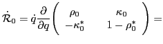$${\dot {\cal R}_0} = {\dot q} \frac {\partial} {\partial q} \Big... ...& \kappa_0 \\ -\kappa_0^{\ast } \quad & 1-\rho_0^{\ast } \end{array}\Bigg) =$$ (35)

$$= \left( \begin{array}{cc} A F B^T - B^\ast F^\ast A^\dagger ~~ ... ...st F^\ast A^\dagger ~~ & B F A^T - A^\ast F^\ast B^\dagger \end{array}\right).$$

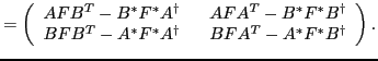
Evaluating the matrix elements of (35) in the canonical basis, we obtain

$$\breve{F}^{i}_{\mu \bar \nu} = \frac {s_{\bar \nu}} {(u_\m... ... \frac {\partial \rho_0} {\partial q_i} \biggr)_{\mu \nu}\,.$$ (36)

By differentiating the HFB equation $[{\cal W}_0, {\cal R}_0] = 0$ with respect to $q_i$, the derivative of the density matrix in (36) can be expressed in terms of the derivatives of the particle-hole and the pairing mean-fields. The resulting 2$\times$2 matrix equation is

$$\bigg[ {\cal A}^\dagger {\dot q_i} \frac {\partial {\cal W}... ... A}, {\cal G} \bigg] + \bigg[ {\cal E}_0, {\cal F} \bigg] = 0.$$ (37)

By employing the properties of $h$ and $\Delta$ with respect to time reversal, we obtain

$$\bigg( \frac {\partial h^\ast} {\partial q_i} \bigg)_{\mu \nu} = s^\ast_{\mu} s_{\nu} \bigg( \frac {\partial h} {\partial q_i} \bigg)_{\bar \mu \bar \nu} \,\,\,,$$ (38)

$$\bigg( \frac {\partial \Delta^\ast} {\partial q_i} \bigg)_{\mu \nu} = s^\ast_{\mu} s^\ast_{\nu} \bigg( \frac {\partial \Delta} {\partial q_i} \bigg)_{\bar \mu \bar \nu},$$ (39)

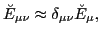
and by approximating the HFB energy matrix in the canonical basis by its diagonal matrix elements,

$$\breve{E}_{\mu\nu} \approx \delta_{\mu\nu}\breve{E}_{\mu},$$ (40)

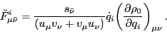
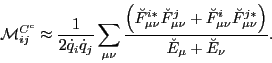
one arrives at an approximate ``BCS-equivalent'' expression for the matrix elements of $F$ in the canonical basis:

$$\breve{F}^{i}_{\mu\nu} \approx \frac{-\dot q_i}{\breve{E}_\m... ...\mu\bar\nu}+\xi^+_{\mu\nu} (\breve{\Delta}^i)_{\mu\nu}\right],$$ (41)

where $x^i\equiv \partial x/\partial q_i$ with $x=\breve h$, $\breve\Delta$, or $\lambda$. In the following, the results obtained by using this approximation will be called ATDHFB-C$^{\rm c}$.

Using relations (40) and (41), the collective mass tensor (34) can now be expressed in terms of the derivatives of the mean-field potentials with respect to the collective coordinates $q_i$ and BCS-like quasiparticle energies (11),

$${\cal M}^{C^{\rm c}}_{ij} \approx \frac {1} {2 {\dot q_i} {... ...{j\ast}_{\mu \nu} \right) } {\breve{E}_\mu + \breve{E}_\nu}.$$ (42)

In the one-dimensional case, the resulting expression agrees with that of Ref. [9].