Time-frequency distribution of energy density

We can visualize the results of MP decomposition in the time-frequency plane by adding Wigner distributions of each of the selected waveforms. The cross Wigner distribution $W[f,h] (t,\omega)$ of functions f and h is defined as

$$W[f,h](t, \omega)=\int f \bigl (t + {\tau \over 2\;} \bigr)... ...l(t- {\tau \over 2} \bigr )\; } e^{- i \omega \tau } d \tau$$ (5)

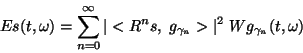
Calculating the Wigner distribution from the whole decomposition as defined by eq. (3) would yield

$$\begin{array}{r} \displaystyle \\ \displaystyle W[s] =... ...; g_{\gamma_m}>} W[g_{\gamma_n}, g_{\gamma_m}] \end{array}$$ (6)

where the double sum gathers the cross terms. In a Wigner distribution of a signal, for which expansion like eq. (3) is not known, cross-terms are not explicitly separable. Minimization of their presence led to the class of Reduced Interference Distributions [14], balancing the tradeoff between resolution and cross-terms contamination. Removing cross-terms from eq. (6) is straightforward--we keep only the first sum, defining the time-frequency distribution of signal's energy as

$$E s (t, \omega) = \sum_{n=0}^\infty \vert<R^n s, \;g_{\gamma_n}>\vert^2 \; W g_{\gamma_n} (t, \omega)$$ (7)

Figure 2 presents decomposition of a simulated signal (plot e, length 500 points) constructed from Gabor functions, sine wave, one-point transient and a chirp (sine with linear frequency modulation). Mentioned structures are drawn separately at the bottom of the figure (a-d). Above the signal we present time-frequency distribution of its energy calculated from the matching pursuit expansion (eq. 7). We observe clear representation of all the structures present in the signal, with exception of the chirp. Changing frequency is explained by a series of structures, since in the Gabor dictionary only waveforms of constant frequency are present.

Figure 2: MP estimates of time-frequency energy distribution of a simulated 500-points signal (e) composed from Gabor functions (a, b), sine, Dirac's delta (c) and chirp (d). Plot (f) presents energy distribution (horizontal time vs. vertical frequency) constructed from a single decomposition in a large ($2*10^6$ atoms) dictionary. Signal is parametrized by 30 waveforms, but changing frequency of the chirp is represented as a series of Gabor functions, since in the Gabor dictionary we have only constant frequency modulations. Middle plot (g) presents average of 100 decompositions of the same signal in different realizations of smaller ($5*10^4$ atoms) stochastic dictionaries. This smoothes the representation of the chirp, but the underlying parametrization is not compact. Upper plot (h)--the same in 3 dimensions. Square root of energy proportional to the height of the surface or "temperature" on 2-dimensional plots.

Upper plots (g and h) of Figure 2 present an application of stochastic dictionaries, which allowed for an improved representation of changing frequency. The same signal (presented below) was decomposed 100 times in different realizations of smaller stochastic dictionary, and resulting energy distributions were averaged. Such a procedure smoothes the representation of the chirp without introducing cross-terms. However, the underlying parametrization is not compact.