


Next: Method of calculations
Up: Theoretical framework
Previous: Additivity of effective s.p.
Determination of effective s.p. observables
Once the averages of physical observables  for the set of
  calculated configurations (
 ) are determined, the
effective s.p. contributions
) are determined, the
effective s.p. contributions
 (19) are found by means of a multivariate least-square fit
(see, e.g., Refs. [29,30]). This is done by minimizing
the function of
defined by
(19) are found by means of a multivariate least-square fit
(see, e.g., Refs. [29,30]). This is done by minimizing
the function of
defined by
![\begin{displaymath}
F\left[o^{\mbox{\rm\scriptsize {eff}}}_{\alpha}\right]=\sum_...
...lpha}^{\mbox{\rm\scriptsize {eff}}} c_{\alpha}(k) \right )^2 .
\end{displaymath}](img127.png) |
(22) |
Note that the problem is only meaningful when the number of configurations
is sufficiently large,  . Following
the general concept of the least-square method,
the partial differentiation with respect to the variables
yields
. Following
the general concept of the least-square method,
the partial differentiation with respect to the variables
yields
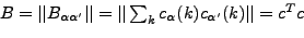
where
 and
and
 . Solving this equation by inverting the
non-singular matrix
. Solving this equation by inverting the
non-singular matrix  gives the solution to the multivariate regression problem:
 |
(24) |
The fact that is positive-definite guarantees that the solution
 corresponds to a minimum of
![$F\left[o^{\mbox{\rm\scriptsize {eff}}}_{\alpha}\right]$](img139.png) .
.
In order to estimate the
variance, we assume that the first statistical moments of residuals,
 |
(25) |
are zero for all  . Consequently,
can be
considered an unbiased estimate of
. Consequently,
can be
considered an unbiased estimate of
 . Furthermore,
under the assumption that
. Furthermore,
under the assumption that
 |
(26) |
for all
 , and
, and
 |
(27) |
for all
 , one can define the
variance-covariance matrix as
, one can define the
variance-covariance matrix as
 , for which the unbiased estimate for
  is given
by
is given
by
 |
(28) |
Finally, the unbiased estimate for the variance-covariance matrix for
is given by
 . In what follows
we do not differentiate between notations for variables and their
estimates.
The least-square procedure described in this section was used to
determine the effective s.p. quadrupole moments
. In what follows
we do not differentiate between notations for variables and their
estimates.
The least-square procedure described in this section was used to
determine the effective s.p. quadrupole moments
 and angular momentum alignments
 .
.
Next: Method of calculations
Up: Theoretical framework
Previous: Additivity of effective s.p.
Jacek Dobaczewski
2007-08-08


